Introduction
How do we estimate the number of people gathered at an event? In football games for instance, one way of estimating the number of spectators is by knowing the number of tickets sold. How about events organised openly for the general public. Events organised at beaches, on the streets, parks, etc. It will definitely help a great deal to automate crowd counting to have a fair idea about the number of people available at the events.
Given a photo of the crowd we can estimate the number of people present. The approach used in this project is from the paper: From Open Set to Closed Set: Supervised Spatial Divide-and-Conquer for Object Counting by Xiong et al. Xiong et al, just like most neural network image processing techniques, basically relies on the excellent feature extraction property of Convolutional Neural Networks (CNNs) to model a probability distribution given image data (density estimation). In their paper, Xiong et al argue that since a sample of image data only represents observable scenes, \(X\), it is difficult for a model to capture a scene count outside \(X\). Hence, they introduce the Supervised Spatial Divide-and-Conquer Network (SS-DCNet) in order to capture unobserved scene counts as well. The idea is to basically leverage on the fact that counting is separable in object space. This intuitively implies that a region can be divided into sub-regions based on a threshold value; each sub-region is counted and the results are accumulated and summed up as the total count.
"Suppose that a network has been trained to accurately predict a closed set of counts, say 0-20. When facing an image with extremely dense objects, one can keep dividing the image into sub images until all sub-region counts are less than 20. The network can then count these sub-images and sum over all local counts to obtain the global image count." [paper]
Method Discussed
In the Spatial Divide-and-Conquer (S-DC) method:
- The image, \(I\), is passed through a pre-trained CNN (eg. VGG16) to obtain the feature map, \(F_0\).
- A closed-set counter predicts the local count value \(C_0\) with \(F_0\) as input. The counter either predicts a single value (Regression-Based Counter) or discretizes and predicts count intervals (Classification-Based Counter).
- \(F_0\) is upsampled by \(\times2\) using a UNet-like decoder to obtain \(F_1\). Each local feature in \(F_1\) corresponds to a sub-region of the input feature map, \(F_0\).
- \(F_1\) is divided and sub-regions are passed through the closed-set counter to predict counts for each sub-region. This produces the first division count, \(C_1\), in the S-DC method.
- A division decider module is then used to select where to divide in each local count, \(DIVC_0\) and \(DIVC_1\) for \(C_0\) and \(C_1\) respectively: $$DIVC_0 = (1-W_1) \circ C_0$$ and $$DIVC_1 = W_1 \circ C_1$$ where \(W_1\) is a matrix initially set to zeros and ones, \(w \in W_1\); \(w \in [0; 1]\) basically to determine which counter input in \(C_1\) is combined with counts \(C_0\). Subsequent parameters of \(W\), \(W_{is}\), are learned. \(\circ\) also denotes the Hadamard product.
- Given the above expressions, both \(C_1\) and \(W_1\) are of the same size, hence the need to upsample \(C_0\) \(\times2\) to the same size, \(\hat{C}_0\). The upsampling process redistributes \(C_0\) to each sub-region, where the sum of \(\hat{C}_0\) should be equal to \(C_0\). A re-distribution map \(U_1\) is therefore computed on features upsampled from \(F_1\) to re-distribute \(C_0\) to its \(\times2\) resolution output, \(\hat{C}_0\). Hence \(\hat{C}_0\) is given by: $$\hat{C}_0 = (C_0 \otimes 1_{2\times2}) \circ U_1$$ $$ \therefore DIVC_0 \rightarrow DIV\hat{C}_0 = (1-W_1) \circ \hat{C}_0$$ where \(\otimes\) denotes the Kronecker product and \(1_{2\times2}\) denotes a \(2\times2\) matrix with all entries equal to 1.
- Finally, the division result, \(DIV\), is given by: $$DIV_1 = DIV\hat{C}_0 + DIVC_1$$ $$DIV_1 = (1-W_1) \circ \hat{C}_0 + W_1 \circ C_1$$
The process is illustrated in \(Fig.1\), below.
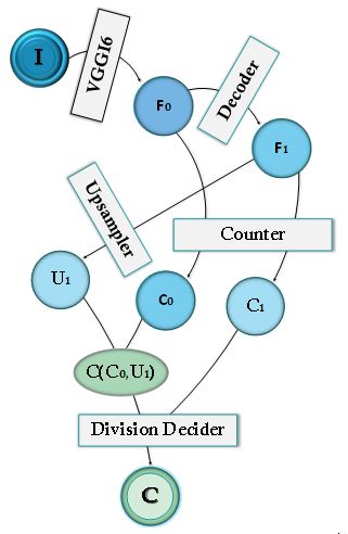
\(Fig.1\). A data flow representation of the single-stage method applied to image \(I\), to generate the final count, \(C\). \(F_0\) is obtained after passing \(I\) through \(VGG16\).\(F_0\) is decoded to \(F_1\). The same counter is applied to both \(F_0\) and \(F_1\) to obtain counts \(C_0\) and \(C_1\) respectively. A division decider is applied to \(C_1\) and upsampled \(C_0\) to obtain the final count \(C\). However, as indicated in the above procedure it is required to add upsampled \(F_1\), \(U_1\), in the upsampling process of \(C_0\).
The above method is known as the single-stage approach to S-DC. It can be extended to a multi-stage S-DC by applying the decoder further to divide the feature map, illustrated in \(Fig.2\). Therefore successive dividers replace proceeding division results until reaching the final decoder block. At this state the final division result, \(DIV_i\), is reached by merging proceeding divisions, \(DIV_{i-1}\), as follows (illustrated in \(Fig.3\)): $$upsampling \rightarrow D\hat{I}V_{i-1} = (DIV_{i-1} \otimes 1_{2\times2}) \circ U_1$$ $$merging \rightarrow DIV_i = (1-W_1) \circ D\hat{I}V_{i-1} + W_1 \circ C_1$$
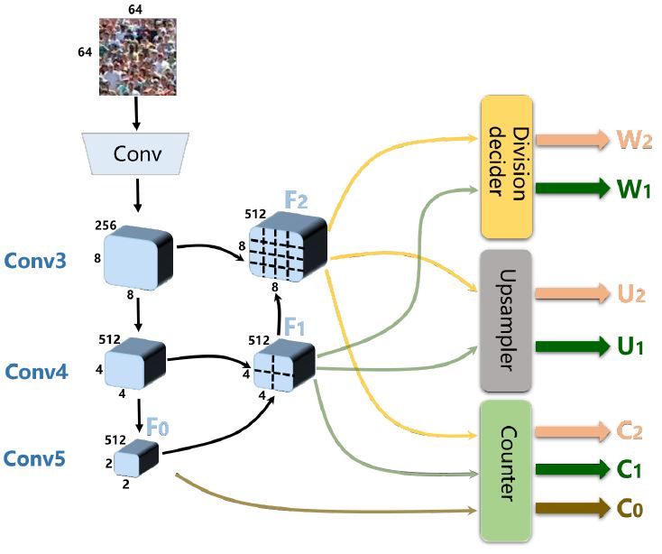
\(Fig.2\) [paper]. An image of size \(64 \times 64\) is passed through the pre-trained network(\(VGG16\)) indicated \(Conv\) to \(F_0\). \(Conv3 - Conv5\) represent the decoder blocks. \(F_1\) is obtained from \(F_0\) and again \(F_0\) is further decoded to \(F_2\). A common counter is applied to all feature maps (\(F_0\), \(F_1\), \(F_2\)) to obtain \(C_0\), \(C_1\) and \(C_2\) respectively. \(F_1\) and \(F_2\) are upsampled to \(U_1\) and \(U_2\) respectively to be added to the resampling processes of preceeding division counts. Initial \(W_{is}\) (\(W_1\) and \(W_2\)) are set for \(F_1\) and \(F_2\) respectively.
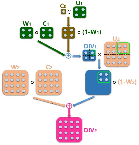
\(Fig.3\) [paper]. In the first part of the division decider, \(DIV\), \(C_0\) is upsampled together with \(U_1\) and passed through the decision decider to generate \(DIV_1\). \(DIV_1\) is upsampled together with \(U_2\) and the decision decider is once again applied to generate \(DIV_2\) which becomes the final count.
Loss Functions
The Loss Function used is based on the mode of closed set counter used; i.e., the Regression-Based Counter or Classification-Based Counter. However, both counters require the summation of individual losses to get the total loss. Losses that are common to both modalities include counter loss (\(L_R\) for regression-based and \(L_C\) for classification based), merge loss (\(L_m\)), upsampling loss (\(L_{up}\)) and division Loss (\(L_{div}\)). A division consistency loss (\(L_{eq}\)) is used only in the regression case basically to ensure consistent counter values.
- \(L_R\), \(L_m\) and \(L_{up}\) all take the form of the \(l_1\) loss which is given by: $$l_1 = \sum _{i=1} ^{n} \mid {C^{gt}, C^{out}}\mid$$ where \(C^{gt}\) denotes the ground-truth count and \(C^{out}\) denotes the output of the individual networks(ie. counter, merge network and upsampler ).
- Cross-entropy loss \(l_c\) is used to compute \(L_C\). Cross-entropy loss is given by: $$l_c\ = -\sum _{l=1} ^{m} C_{ob} \log (p_{ob},c)$$ where \(m\) denotes the number of classes, \(C\) denotes binary indicator (0 or 1) ie., if class label \(c\) is the correct classification for observation \(ob\) and \(p\) denotes predicted probability observation \(ob\) is of class \(c\).
- \(L_{div}\) is given by: $$L_{div}^{i} = -\sum _{j=1} ^{H_i} \sum _{k=1} ^{W_i} 1\left\{C_{i-1}^{gt}[j,k]>C_{max}\right\} \times $$ \[\qquad \qquad log (\max(W_i[2_j-1:2_j,2_k-1:2_k])\] where \(C_{i-1}^{gt}[j,k]\) denotes the element of the \(j-th\) row and the \(k-th\) column of \(C_{i-1}^{g}t\), and \(W_i[2_j-1:2_j,2_k-1:2_k]\) the elements lying in the \((2_j-1)-th\) to \(2_j-th\) row, \((2_k-1)-th\) to \(2_k-th\) column of \(W_i\) [paper].
- \(L_{eq}\) is given by: $$L_{eq}^{i} = -\sum _{j=1} ^{H_{i-1}} \sum _{k=1} ^{W_{i-1}} 1\left\{C_{i-1}^{gt}[j,k]>C_{max}\right\} \times \mid C_{i=1}[j,k] - $$ \[\qquad \qquad sum(C_i[2_j-1:2_j,2_k-1:2_k])\mid\] where \(sum\) is the operator that returns the sum of all elements[paper].
Regression-Based Counter Loss
The overall Regression-Based Counter Loss \(L_{reg}\) is given by: $$L_{reg} = L_R + L_m + L_{up} + L_{div} + L_{eq}$$ $$L_{reg} = \sum _{i=0}^{N}[L_R + L_m +L_{up} + L_{div} + L_{eq}]$$Classification-Based Counter Loss
The overall Classification-Based Counter Loss, \(L_{cls}\) is given by: $$L_{cls} = L_C + L_m + L_{up} + L_{div}$$ $$L_{cls} = \sum _{i=0}^{N}[L_R + L_m + L_{up} + L_{div}]$$ The details of individual losses are covered in the paper.Results
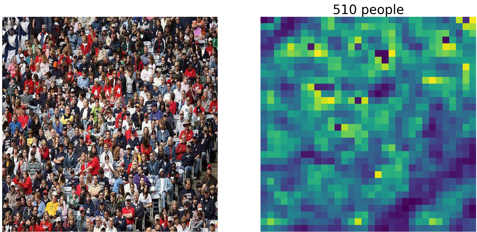
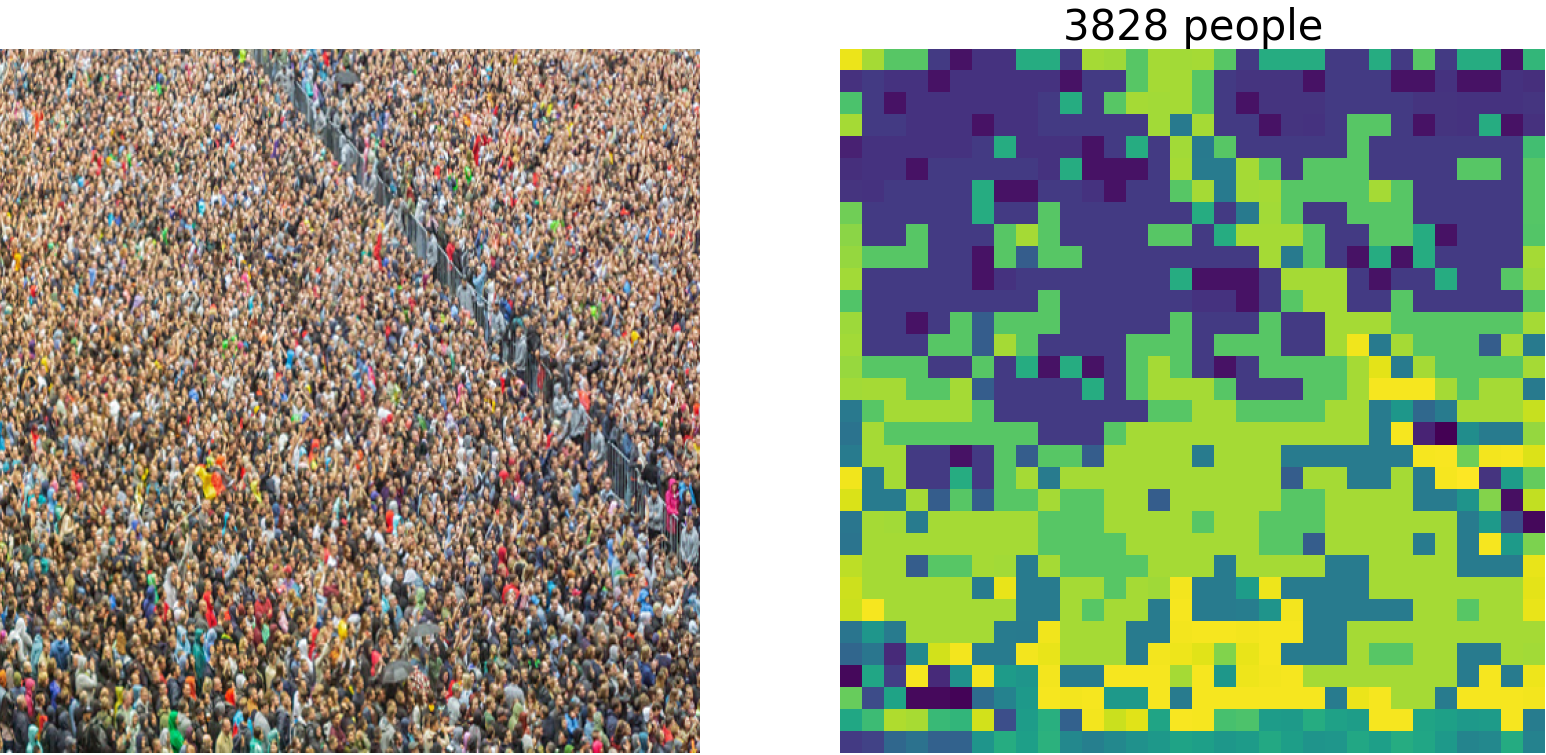
In the experiment, test photos were taken from pixabay; for copyright reasons. The codes and models were obtained from the authors' repository. Pre-trained weights of the model trained on the ShanghaiTech Part_B crowd counting dataset was applied to the following images to estimate their respective counts from final division decider outputs.
Copyright Free images downloaded from pixabay
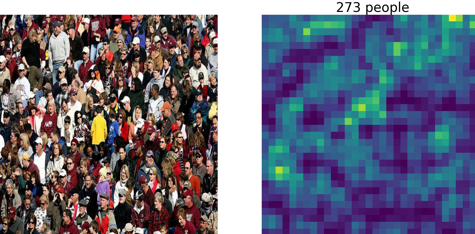
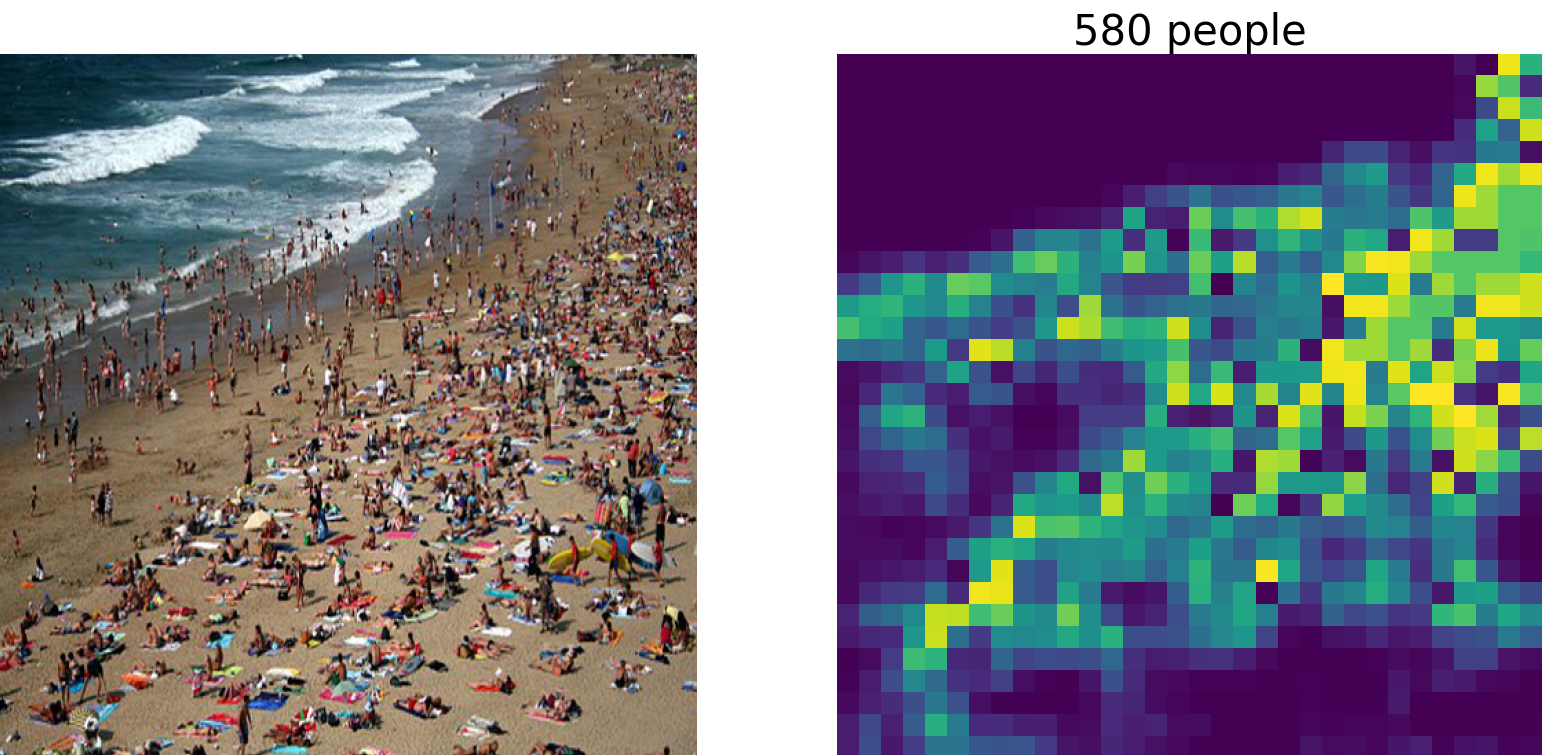
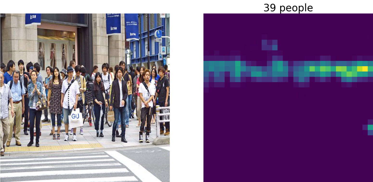
Copyright Free images downloaded from pixabay
↑ Back to Top