Introduction
This project is inspired by the paper: Unsupervised Feature Learning for Online Voltage Stability Evaluation and Monitoring based on Variational Autoencoder (VAE). In their paper, Yang et al explored the potential of a probabilistic learning approach for online monitoring of voltage stability. They trained a Variational Autoencoder on Phasor Measurement Unit (PMU) monitoring data. The effectiveness and accuracy of their approach was then compared with other approaches via simulation. The simulation was basically based on power systems with different load increment models.
Their goal was to capture crucial features that appropriately model the load changing trend as it is a significant factor in voltage stability. However the paper suggests making direct approximation to model the load changing trend is complicated. So they decided to learn low-dimensional features from voltage measurements. This data manifold learning approach they believed could appropriately capture the unknown load profile. Hence, the unknown load profile is treated as a latent variable. The idea of latent variable is, in a way, to represent a data generation process. In other words all observed variables have a "common cause" which is implicitly represented by the latent variable. Unsupervised probabilistic approximation with latent variables usually require methods including Expectation Maximisation, Markov Chain Monte Carlo and Variational Bayes. However, Yang et al indicated that modelling the relation involving nonlinear power equation flow is complex; hence applying the aforementioned methods is computationally intractable. Hence they use deep learning approach analogous to Variational Bayes, i.e. Variational Autoencoder.
Method Used
In this project, I adopt their method for approximating latent variable via VAE to monitor electric voltage stability using Electrical Grid Stability Simulated Data Set dataset from UCI Machine Learning Repository. The data consists of 14 features with 10000 training examples. Each training example is labelled as stable or unstable. However, in training, I only used the stable examples. The method is simply to learn the latent variable for the stable features and regenerate the probability distribution of the stable features. Hence, applying the model parameters to stable input signal outside the training data, should produce closely related distribution and unstable signal yielding negative results.
Since we are dealing with structured data, the network architecture used only fully connected layers. The network details and architecture is as follows:
- Size of features: 2172 x 13 train set and 724 x 13 validation set
- Number of Encoder layers: 3 with 2 representing statistics from sample distribution
- Number of Decoder layers: 2
- Input Layer output dimension: 64
- Output Dimension of Latent Variable: 32
- Optimizer: adam with 1x10⁻⁴ learning rate
- Batch Size: 32
Method Discussed in Detail
The idea of VAE is basically to optimize: $$\mathcal{L} (\theta,\phi; x^{(i)}) = -D_{KL}(q_\phi(z|x^{(i)})||p_\theta(z) +$$ \[\qquad \qquad E_{q_\phi(z|x^{(i)})}[\log p_\theta(x^{(i)}|z)]\] w.r.t \(\theta\) and \(\phi\), where;
- x = observed variable
- z = latent variable
- \(\theta\) = variational parameter
- \(\phi\) = generative parameter
- \(\mathcal{L}\) = Evidence Lower Bound (ELBO)
- \(D_{KL}\) = Kullback-Leibler Divergence
- \(p_\theta\) = distribution defined over the observed variables
- \(q_\phi\) = distribution defined over the latent variables
However due to inconvenience in computing gradient w.r.t \(\phi\), the Monte Carlo gradient estimator, which is an alternative, is in effect impractical. Hence, the approach used in VAE is to reparameterize \(q_\phi\) (z|x) with a differentiable transformation \(g_\phi(\epsilon, x)\), where \(\epsilon\) is an auxiliary noise variable.The Monte Carlo gradient estimator is given by: $$\nabla_\phi E_{q_\phi} [f(z)] \simeq \frac{1}{L} \sum _{l=1} ^{L} f(z) \nabla_{q_\phi z^{(l)}} \log q_\phi (z^{(l)})$$ where \(z^{(l)} \sim q_\phi (z|x^{(i)})\). Applying the reparameterized form yields: $$ E_{q_\phi(z|x^{(i)})} [f(z)] \simeq \frac{1}{L} \sum _{l=1} ^{L} f(g_\phi (\epsilon^{(l)} ,x^{(i)})) $$ where \(\epsilon^{(l)} \sim p(\epsilon)\). Hence the evidence lower bound is given by: $$\mathcal{L}(\theta,\phi; x^{(i)}) = -D_{KL}(q_\phi(z|x^{(i)})||p_\theta(z) + $$ \[\qquad \qquad \frac{1}{L} \sum (\log p_\phi (x^{(l)}|z^{(i,l)}))\] where \(z^{(i,l)} \sim g_\phi (\epsilon^{(i,l)}|x^{(i)})\) and \(\epsilon^{(l)} \sim p(\epsilon)\).
In summary, VAE just like vanilla Autoencoder comprise the encoder step during which features are downsampled and decoder step in which the features are upsampled to regenerate features drawn from the original data generating process. However, VAE, as opposed to vanilla Autoencoders, involves drawing samples from the distribution of the downsampled data for the decoding process. Hence the encoder step involves a generative process that takes latent variables as input and outputs the parameters for a conditional distribution of the observed variable. Whereas the decoder step involves an inference process which takes an observed variable as input and outputs parameters that define the conditional distribution of the latent profile.
Encoder step:
$$ Generative = p(x|z) $$
Decoder Step:
$$ Inference = p(z|x) $$
Training the VAE involves maximizing the ELBO on the marginal log-likelihood:
$$ \log(p(x)) = \log(\sum_zp(x,z)) = \mathcal{L}(q)+D_{KL} (q||p) $$
It is observed that maximizing the ELBO \((\mathcal{L}(q))\), monotonically increases the log-likelihood of the observed data and in effect decreases the Kullback-Leibler Divergence \((D_{KL} (q||p))\) which in simple terms measures the difference between distribution of the "actual" or reference data generating process and that of the model. The optimization process is then carried out using sample Monte Carlo estimate of the expectation: $$ \log p(x|z)+\log p(z) - \log q(z|x) $$ where z is sampled from \(q(z|x)\) (reparameterization trick).
With regards to monitoring voltage stability, the lower bound is computed on test input variables not used in the training process using the learned model parameters. The results is then compared with the outputs obtained from the validation dataset used in training. By so doing every input with a lower bound close to that obtained from the model is considered stable and unstable otherwise.
Results
In the experiment, test samples were taken from same dataset but were not used for training. The lower bound was computed for both inputs known to be stable and inputs known to be unstable (see figure below). The values computed on the stable signal yielded results close to the model outputs on the validation set. However, the difference between the unstable sample and the model results was very huge; which indicates instability in the network. The codes and pre-trained weights for the model are available on the project's repository.
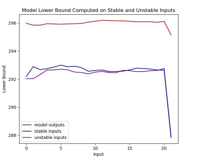
Lower bound values computed on unstable inputs, indicated in red, show how they are unrelated to the model outputs (purple). In contrast, the values from the stable inputs, shown in blue, are close to the model outputs.
↑ Back to Top